Part 8: Summary exercises - SOLVED
Contents
Part 8: Summary exercises - SOLVED#
This workbook does requires the titanic and avocado datasets. As usual you will need to import numpy and pandas
# Use this cell to import numpy and pandas
import numpy as np
import pandas as pd
# Use this cell to import the titanic dataset.
df_titanic = pd.read_excel("titanic.xlsx")
df_avocado = pd.read_excel("avocado.xlsx")
Exercise 8.1#
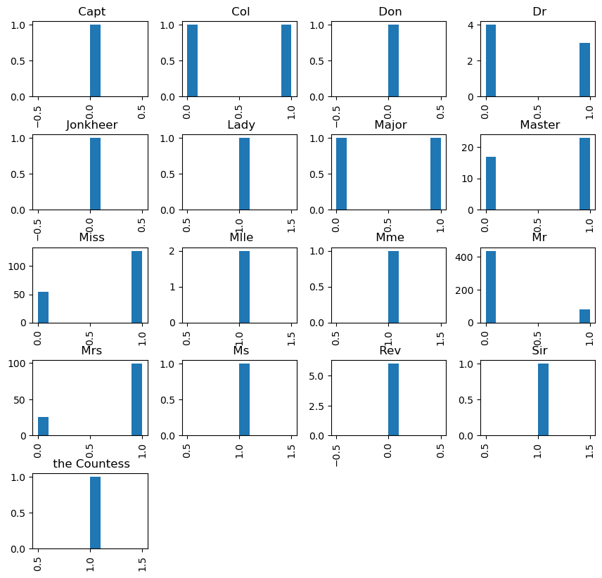
We will be processing the titanic.xlsx spreadsheet. Your task is to extract the title each passenger gave (e.g. Miss, Mr etc.) from the Name column and saved its value in the new column title.
After you succeed plot the histogram of Survived by the groups in Title. You should investigate whether the title that somebody used affected if they were more likely to survive.
Hint use: your_data_frame["Your Column"].str.split(' ')
To make your histograms readable add the parameter figsize=(10, 10) to your plotting function.
titanic_name = df_titanic.Name.str.replace(".", "|")
titanic_name = titanic_name.str.replace(",", "|")
titanic_name = titanic_name.str.split("|")
print(titanic_name)
0                            [Braund,  Mr,  Owen Harris]
1      [Cumings,  Mrs,  John Bradley (Florence Briggs...
2                             [Heikkinen,  Miss,  Laina]
3       [Futrelle,  Mrs,  Jacques Heath (Lily May Peel)]
4                           [Allen,  Mr,  William Henry]
                             ...
886                            [Montvila,  Rev,  Juozas]
887                     [Graham,  Miss,  Margaret Edith]
888         [Johnston,  Miss,  Catherine Helen "Carrie"]
889                            [Behr,  Mr,  Karl Howell]
890                              [Dooley,  Mr,  Patrick]
Name: Name, Length: 891, dtype: object
titanic_title  = pd.Series([item[1] for item in titanic_name])
titanic_title.unique()
array([' Mr', ' Mrs', ' Miss', ' Master', ' Don', ' Rev', ' Dr', ' Mme',
       ' Ms', ' Major', ' Lady', ' Sir', ' Mlle', ' Col', ' Capt',
       ' the Countess', ' Jonkheer'], dtype=object)
df_titanic["Title"] = titanic_title
df_titanic.head()
| PassengerId | Name | Sex | Age | Ticket | Fare | Cabin | Survived | Title | |
|---|---|---|---|---|---|---|---|---|---|
| 0 | 1 | Braund, Mr. Owen Harris | male | 22.0 | A/5 21171 | 7.2500 | NaN | 0 | Mr |
| 1 | 2 | Cumings, Mrs. John Bradley (Florence Briggs Th... | female | 38.0 | PC 17599 | 71.2833 | C85 | 1 | Mrs |
| 2 | 3 | Heikkinen, Miss. Laina | female | 26.0 | STON/O2. 3101282 | 7.9250 | NaN | 1 | Miss |
| 3 | 4 | Futrelle, Mrs. Jacques Heath (Lily May Peel) | female | 35.0 | 113803 | 53.1000 | C123 | 1 | Mrs |
| 4 | 5 | Allen, Mr. William Henry | male | 35.0 | 373450 | 8.0500 | NaN | 0 | Mr |
df_titanic.hist(column="Survived", by="Title", figsize=(10, 10));
Exercise 8.2#
This exercise is also about the tititanic data.
When we plotted the correlation matrix, we noticed that the displayed columns were only numerical. To convert a column whose values are categorical (e.g. in this dataset the Sex column has two categories male and female).
We can use
pd.factorize(your_data_frame_object)
this will put the integers values to represent each category. If there are two categories we would get 0 and 1.
You task is to create a new column that represents Sex numerically via using pd.factorize.
Then display the correlation matrix of your new data frame. Which column has the highest correlation with the column Survived (apart from Survived itself).
num_sex = pd.factorize(df_titanic.Sex)
num_sex
(array([0, 1, 1, 1, 0, 0, 0, 0, 1, 1, 1, 1, 0, 0, 1, 1, 0, 0, 1, 1, 0, 0,
        1, 0, 1, 1, 0, 0, 1, 0, 0, 1, 1, 0, 0, 0, 0, 0, 1, 1, 1, 1, 0, 1,
        1, 0, 0, 1, 0, 1, 0, 0, 1, 1, 0, 0, 1, 0, 1, 0, 0, 1, 0, 0, 0, 0,
        1, 0, 1, 0, 0, 1, 0, 0, 0, 0, 0, 0, 0, 1, 0, 0, 1, 0, 1, 1, 0, 0,
        1, 0, 0, 0, 0, 0, 0, 0, 0, 0, 1, 0, 1, 0, 0, 0, 0, 0, 1, 0, 0, 1,
        0, 1, 0, 1, 1, 0, 0, 0, 0, 1, 0, 0, 0, 1, 0, 0, 0, 0, 1, 0, 0, 0,
        1, 1, 0, 0, 1, 0, 0, 0, 1, 1, 1, 0, 0, 0, 0, 1, 0, 0, 0, 1, 0, 0,
        0, 0, 1, 0, 0, 0, 0, 1, 0, 0, 0, 0, 1, 1, 0, 0, 0, 0, 1, 0, 0, 0,
        0, 1, 0, 0, 1, 0, 0, 0, 1, 0, 1, 0, 0, 0, 1, 0, 1, 0, 1, 1, 0, 0,
        1, 1, 0, 0, 0, 0, 0, 1, 0, 0, 1, 0, 0, 1, 0, 0, 0, 1, 1, 0, 1, 0,
        0, 0, 0, 0, 0, 0, 0, 0, 0, 1, 1, 0, 0, 1, 0, 1, 0, 1, 0, 0, 1, 1,
        0, 0, 0, 0, 1, 1, 0, 0, 0, 1, 0, 0, 1, 1, 1, 1, 1, 1, 0, 0, 0, 0,
        1, 0, 0, 0, 1, 1, 0, 0, 1, 0, 1, 1, 1, 0, 0, 1, 0, 0, 0, 0, 0, 0,
        0, 0, 0, 1, 1, 1, 0, 1, 0, 0, 0, 1, 0, 1, 1, 0, 0, 1, 0, 0, 1, 1,
        0, 1, 1, 1, 1, 0, 0, 1, 1, 0, 1, 1, 0, 0, 1, 1, 0, 1, 0, 1, 1, 1,
        1, 0, 0, 0, 1, 0, 0, 1, 0, 0, 0, 1, 0, 0, 0, 1, 1, 1, 0, 0, 0, 0,
        0, 0, 0, 0, 1, 1, 1, 1, 0, 0, 1, 0, 0, 0, 1, 1, 1, 1, 0, 0, 0, 0,
        1, 1, 1, 0, 0, 0, 1, 1, 0, 1, 0, 0, 0, 1, 0, 1, 0, 0, 0, 1, 1, 0,
        1, 0, 0, 1, 0, 0, 1, 0, 1, 0, 0, 0, 0, 1, 0, 0, 1, 0, 0, 1, 1, 1,
        0, 1, 0, 0, 0, 1, 0, 0, 1, 1, 0, 0, 0, 1, 1, 0, 0, 1, 1, 1, 0, 0,
        1, 0, 0, 1, 0, 0, 1, 0, 1, 0, 0, 0, 0, 0, 0, 0, 0, 1, 1, 0, 0, 0,
        0, 0, 0, 0, 0, 0, 0, 1, 0, 0, 1, 1, 1, 0, 0, 0, 0, 1, 0, 0, 0, 1,
        0, 1, 1, 0, 0, 0, 0, 0, 0, 0, 0, 0, 1, 0, 1, 0, 0, 1, 1, 1, 1, 0,
        1, 0, 0, 0, 0, 0, 0, 1, 0, 0, 1, 0, 1, 0, 1, 0, 0, 1, 0, 0, 1, 0,
        0, 0, 1, 0, 0, 1, 1, 1, 0, 1, 0, 1, 1, 1, 1, 0, 0, 0, 1, 0, 0, 0,
        0, 0, 0, 0, 1, 0, 1, 0, 1, 1, 0, 0, 0, 0, 1, 0, 0, 1, 0, 0, 0, 1,
        0, 1, 0, 0, 1, 1, 1, 0, 1, 1, 0, 0, 0, 1, 0, 0, 0, 0, 0, 1, 0, 1,
        0, 0, 1, 0, 0, 0, 1, 0, 0, 0, 0, 0, 0, 0, 1, 1, 1, 0, 1, 0, 0, 1,
        0, 1, 1, 0, 0, 0, 0, 0, 0, 0, 0, 1, 0, 0, 0, 0, 0, 0, 1, 1, 0, 0,
        1, 0, 0, 1, 1, 0, 1, 0, 0, 0, 0, 1, 0, 1, 0, 1, 1, 0, 0, 1, 0, 0,
        0, 0, 0, 0, 0, 0, 0, 0, 0, 1, 1, 0, 0, 0, 0, 0, 0, 1, 1, 0, 1, 0,
        0, 0, 0, 0, 0, 0, 0, 1, 0, 1, 0, 0, 0, 0, 0, 1, 0, 0, 1, 0, 1, 0,
        0, 0, 1, 0, 1, 0, 1, 0, 0, 0, 0, 0, 1, 1, 0, 0, 1, 0, 0, 0, 0, 0,
        1, 1, 0, 1, 1, 0, 0, 0, 0, 0, 1, 0, 0, 0, 0, 0, 1, 0, 0, 0, 0, 1,
        0, 0, 1, 0, 0, 0, 1, 0, 0, 0, 0, 1, 0, 0, 0, 1, 0, 1, 0, 1, 0, 0,
        0, 0, 1, 0, 1, 0, 0, 1, 0, 1, 1, 1, 0, 0, 0, 0, 1, 0, 0, 0, 0, 0,
        1, 0, 0, 0, 1, 1, 0, 1, 0, 1, 0, 0, 0, 0, 0, 1, 0, 1, 0, 0, 0, 1,
        0, 0, 1, 0, 0, 0, 1, 0, 0, 1, 0, 0, 0, 0, 0, 1, 1, 0, 0, 0, 0, 1,
        0, 0, 0, 0, 0, 0, 1, 0, 0, 0, 0, 0, 0, 1, 0, 0, 1, 1, 1, 1, 1, 0,
        1, 0, 0, 0, 1, 1, 0, 1, 1, 0, 0, 0, 0, 1, 0, 0, 1, 1, 0, 0, 0, 1,
        1, 0, 1, 0, 0, 1, 0, 1, 1, 0, 0]),
 Index(['male', 'female'], dtype='object'))
df_titanic["NumericalSex"] = num_sex[0]
df_titanic.corr(numeric_only=True)
| PassengerId | Age | Fare | Survived | NumericalSex | |
|---|---|---|---|---|---|
| PassengerId | 1.000000 | 0.036847 | 0.012658 | -0.005007 | -0.042939 |
| Age | 0.036847 | 1.000000 | 0.096067 | -0.077221 | -0.093254 |
| Fare | 0.012658 | 0.096067 | 1.000000 | 0.257307 | 0.182333 |
| Survived | -0.005007 | -0.077221 | 0.257307 | 1.000000 | 0.543351 |
| NumericalSex | -0.042939 | -0.093254 | 0.182333 | 0.543351 | 1.000000 |
NumericalSex column is highly correlated with Survived column, the correlation is 0.54.
Exercise 8.3#
You are an advisor of a restaurant that is famous from making Poached eggs with smashed avocado. The restaurant plans to open a new branch, but it cannot decide on the region (it considers all available regions from avocado.xlsx). You are asked to make some suggestions. You thought that it may be best to open a restaurant where on average the avocado prices are the lowest.
From the avocado.xlsx find out which region has on average the cheapest (lowest AveragePrice) avocado.
Hint: Use groupby
df_avocado.head()
| Date | AveragePrice | Total Volume | 4046 | 4225 | 4770 | Total Bags | Small Bags | Large Bags | XLarge Bags | type | year | region | |
|---|---|---|---|---|---|---|---|---|---|---|---|---|---|
| 0 | 2015-12-27 | 1.33 | 64236.62 | 1036.74 | 54454.85 | 48.16 | 8696.87 | 8603.62 | 93.25 | 0.0 | conventional | 2015 | Albany |
| 1 | 2015-12-20 | 1.35 | 54876.98 | 674.28 | 44638.81 | 58.33 | 9505.56 | 9408.07 | 97.49 | 0.0 | conventional | 2015 | Albany |
| 2 | 2015-12-13 | 0.93 | 118220.22 | 794.70 | 109149.67 | 130.50 | 8145.35 | 8042.21 | 103.14 | 0.0 | conventional | 2015 | Albany |
| 3 | 2015-12-06 | 1.08 | 78992.15 | 1132.00 | 71976.41 | 72.58 | 5811.16 | 5677.40 | 133.76 | 0.0 | conventional | 2015 | Albany |
| 4 | 2015-11-29 | 1.28 | 51039.60 | 941.48 | 43838.39 | 75.78 | 6183.95 | 5986.26 | 197.69 | 0.0 | conventional | 2015 | Albany |
df_avocado_grouped = df_avocado.groupby("region").mean(numeric_only=True)
df_avocado_grouped.head()
| AveragePrice | Total Volume | 4046 | 4225 | 4770 | Total Bags | Small Bags | Large Bags | XLarge Bags | year | |
|---|---|---|---|---|---|---|---|---|---|---|
| region | ||||||||||
| Albany | 1.561036 | 47537.869734 | 1824.081775 | 37621.208254 | 162.832337 | 7929.747367 | 6647.765473 | 1153.496213 | 128.488639 | 2016.147929 |
| Atlanta | 1.337959 | 262145.322041 | 146116.867959 | 31218.510385 | 311.385769 | 84498.560888 | 51605.727337 | 32070.044556 | 822.786036 | 2016.147929 |
| BaltimoreWashington | 1.534231 | 398561.891479 | 35656.218166 | 245982.888876 | 12466.730976 | 104456.053462 | 100939.683195 | 2903.984586 | 612.382722 | 2016.147929 |
| Boise | 1.348136 | 42642.567308 | 20019.507604 | 3461.682367 | 3186.787840 | 15974.592456 | 13840.037249 | 2103.634083 | 30.915207 | 2016.147929 |
| Boston | 1.530888 | 287792.854527 | 4994.610059 | 214219.864290 | 4982.294970 | 63596.085207 | 58906.590355 | 4438.364704 | 251.124231 | 2016.147929 |
df_avocado_grouped_sorted = df_avocado_grouped.sort_values(by=["AveragePrice"])
df_avocado_grouped_sorted.head()
| AveragePrice | Total Volume | 4046 | 4225 | 4770 | Total Bags | Small Bags | Large Bags | XLarge Bags | year | |
|---|---|---|---|---|---|---|---|---|---|---|
| region | ||||||||||
| Houston | 1.047929 | 6.010884e+05 | 2.951861e+05 | 141196.545858 | 16140.446805 | 148565.278166 | 96228.305740 | 51372.082633 | 964.889793 | 2016.147929 |
| DallasFtWorth | 1.085592 | 6.166251e+05 | 3.270901e+05 | 139557.675828 | 12492.822811 | 137484.475000 | 120774.367101 | 15431.128373 | 1278.973609 | 2016.147929 |
| SouthCentral | 1.101243 | 2.991952e+06 | 1.582963e+06 | 652218.952781 | 66259.744793 | 690510.160799 | 546791.372249 | 135907.808846 | 7810.979704 | 2016.147929 |
| CincinnatiDayton | 1.209201 | 1.317219e+05 | 5.411698e+03 | 61058.899290 | 3421.026598 | 61828.161065 | 16751.165444 | 44296.434290 | 780.564290 | 2016.147929 |
| Nashville | 1.212101 | 1.053612e+05 | 5.381327e+04 | 11273.696450 | 1909.847426 | 38364.397663 | 29712.387101 | 8322.172811 | 329.840710 | 2016.147929 |
your_recommendation = df_avocado_grouped_sorted.index[0]
print(f"Your recommendation to the restaurant is {your_recommendation}")
Your recommendation to the restaurant is Houston