APPENDIX

Code used to make plots embedded in notebook

import numpy as np
import matplotlib.pyplot as plt

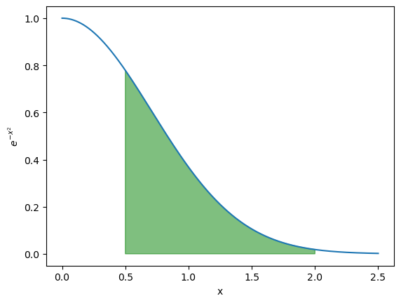
x_range = np.linspace(0,2.5,1000000) # Lots of points on x axis to make line smooth!
y_vals = np.exp(-x_range**2) # e^{-x^2} for all points in x

# Find only those points within the range of the integral
vals_to_be_integrated = (x_range>0.5) & (x_range<2)
x_range_to_be_integrated = x_range[vals_to_be_integrated]
y_vals_to_be_integrated = y_vals[vals_to_be_integrated]

plt.plot(x_range, y_vals) # Plot the line
plt.fill([0.5] + list(x_range_to_be_integrated) + [2],
         [0] + list(y_vals_to_be_integrated) + [0], alpha=0.5, color='green') # Highlights the region to be integrated in green with semi-transparency
plt.plot()
plt.xlabel('x')
plt.ylabel('$e^{-x^2}$')

Text(0, 0.5, '$e^{-x^2}$')

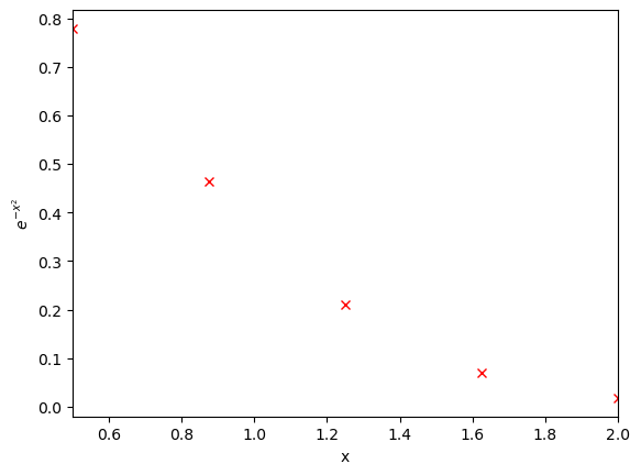
x_range = np.linspace(0.5,2,5)
y_vals = np.exp(-x_range**2)

plt.plot(x_range, y_vals, 'rx') # Plot the line
plt.plot()
plt.xlabel('x')
plt.ylabel('$e^{-x^2}$')
plt.xlim(0.5,2.0)

(0.5, 2.0)

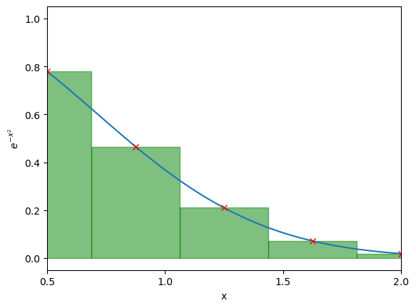
x_range_full = np.linspace(0,2.5,1000000) # Lots of points on x axis to make line smooth!
y_vals_full = np.exp(-x_range_full**2) # e^{-x^2} for all points in x
plt.plot(x_range_full, y_vals_full) # Plot the line

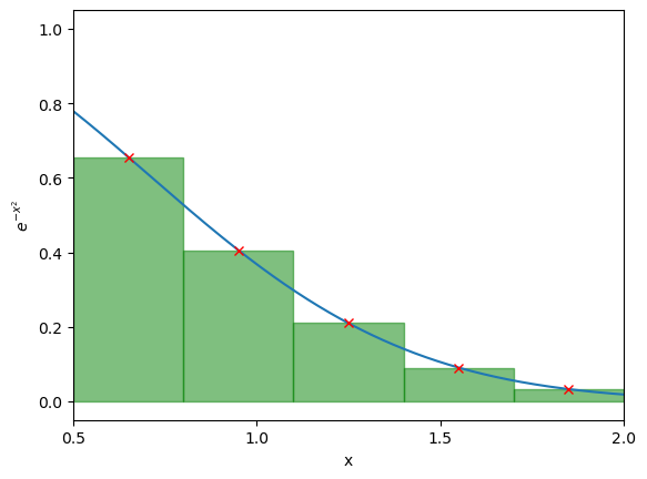
x_range = np.linspace(0.5,2,5)
y_vals = np.exp(-x_range**2)

plt.plot(x_range, y_vals, 'rx') # Plot the line
# plot the rectangles
x_step = x_range[1] - x_range[0]
for x,y in zip(x_range, y_vals): # zip lets me iterate over two lists together
    plt.fill([x-x_step/2, x-x_step/2, x+x_step/2, x+x_step/2],
             [0, y, y, 0], alpha=0.5, color='green', linestyle='-')
plt.plot()
plt.xlabel('x')
plt.ylabel('$e^{-x^2}$')
plt.xlim(0.5,2)
plt.xticks([0.5,1,1.5,2])

([<matplotlib.axis.XTick at 0x12cbcba00>,
  <matplotlib.axis.XTick at 0x12cbcbbe0>,
  <matplotlib.axis.XTick at 0x12cbc33d0>,
  <matplotlib.axis.XTick at 0x12cc301f0>],
 [Text(0.5, 0, '0.5'),
  Text(1.0, 0, '1.0'),
  Text(1.5, 0, '1.5'),
  Text(2.0, 0, '2.0')])

x_range_full = np.linspace(0,2.5,1000000) # Lots of points on x axis to make line smooth!
y_vals_full = np.exp(-x_range_full**2) # e^{-x^2} for all points in x
plt.plot(x_range_full, y_vals_full) # Plot the line


temp_x_range = np.linspace(0.5,2,6)
x_range = (temp_x_range[0:-1] + temp_x_range[1:]) / 2. # What am I doing here??
y_vals = np.exp(-x_range**2)

plt.plot(x_range, y_vals, 'rx') # Plot the line
# plot the rectangles
x_step = temp_x_range[1] - temp_x_range[0]
for x,y in zip(x_range, y_vals): # zip lets me iterate over two lists together
    plt.fill([x-x_step/2, x-x_step/2, x+x_step/2, x+x_step/2],
             [0, y, y, 0], alpha=0.5, color='green', linestyle='-')
plt.plot()
plt.xlabel('x')
plt.ylabel('$e^{-x^2}$')
plt.xlim(0.5,2)
plt.xticks([0.5,1,1.5,2])

([<matplotlib.axis.XTick at 0x12cc6a850>,
  <matplotlib.axis.XTick at 0x12cc6a970>,
  <matplotlib.axis.XTick at 0x12cc6a220>,
  <matplotlib.axis.XTick at 0x12d5d15b0>],
 [Text(0.5, 0, '0.5'),
  Text(1.0, 0, '1.0'),
  Text(1.5, 0, '1.5'),
  Text(2.0, 0, '2.0')])

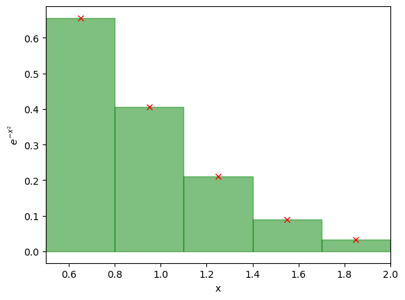
temp_x_range = np.linspace(0.5,2,6)
x_range = (temp_x_range[0:-1] + temp_x_range[1:]) / 2. # Can you figure out what this line is doing??
y_vals = np.exp(-x_range**2)

plt.plot(x_range, y_vals, 'rx') # Plot the line
# plot the rectangles and compute area
x_step = temp_x_range[1] - temp_x_range[0]
current_area = 0
for x,y in zip(x_range, y_vals): # zip lets me iterate over two lists together
    plt.fill([x-x_step/2, x-x_step/2, x+x_step/2, x+x_step/2],
             [0, y, y, 0], alpha=0.5, color='green', linestyle='-')
    current_area += x_step * y
plt.plot()
plt.xlabel('x')
plt.ylabel('$e^{-x^2}$')
plt.xlim(0.5,2)
print(f"I have computed the integral to be {current_area}")

I have computed the integral to be 0.4181083032593553

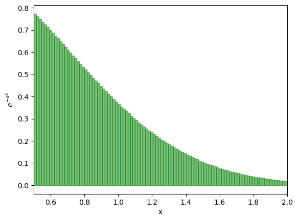
temp_x_range = np.linspace(0.5,2,101)
x_range = (temp_x_range[0:-1] + temp_x_range[1:]) / 2. # Can you figure out what this line is doing??
y_vals = np.exp(-x_range**2)

#plt.plot(x_range, y_vals, 'rx') # Plot the line
# plot the rectangles and compute area
x_step = temp_x_range[1] - temp_x_range[0]
current_area = 0
for x,y in zip(x_range, y_vals): # zip lets me iterate over two lists together
    plt.fill([x-x_step/2, x-x_step/2, x+x_step/2, x+x_step/2],
             [0, y, y, 0], alpha=0.5, color='green', linestyle='-')
    current_area += x_step * y
plt.plot()
plt.xlabel('x')
plt.ylabel('$e^{-x^2}$')
plt.xlim(0.5,2)
print(f"I have computed the integral to be {current_area}")

I have computed the integral to be 0.4207937696440889

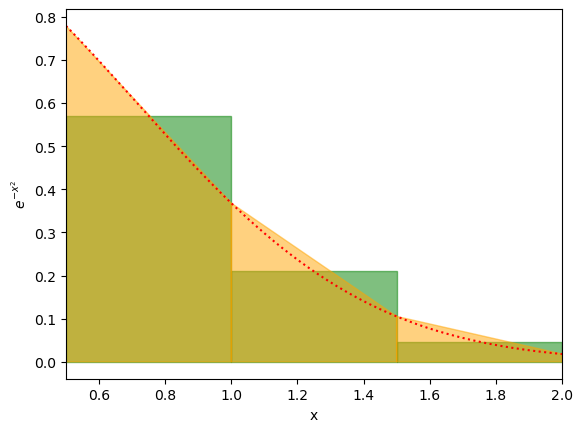
# Let's add the rectangles first. THIS IS CODE FROM BEFORE
num_shapes = 3


edges_x_range = np.linspace(0.5,2,num_shapes+1)
x_range = (edges_x_range[0:-1] + edges_x_range[1:]) / 2. # Can you figure out what this line is doing??
y_vals = np.exp(-x_range**2)

# Plot the actual line
full_x_range = np.linspace(0.5,2,100000)
full_y_vals = np.exp(-full_x_range**2)
plt.plot(full_x_range, full_y_vals, 'r:') # Plot the line


# plot the rectangles
x_step = edges_x_range[1] - edges_x_range[0]
for x,y in zip(x_range, y_vals): # zip lets me iterate over two lists together
    plt.fill([x-x_step/2, x-x_step/2, x+x_step/2, x+x_step/2],
             [0, y, y, 0], alpha=0.5, color='green', linestyle='-')
plt.plot()

# Now let's add the trapeziums. THIS IS THE NEW CODE
y_vals_trapezium = np.exp(-edges_x_range**2)
for i in range(len(edges_x_range) - 1):
    # Identify the corners of the trapezium, a left edge, right edge, topleft y value, topright y value and bottom y value (0 in all cases)
    left_edge = edges_x_range[i]
    right_edge = edges_x_range[i+1]
    bottom_y_value = 0
    topleft_y_value = y_vals_trapezium[i]
    topright_y_value = y_vals_trapezium[i+1]
    # Draw the trapezium
    plt.fill([left_edge, left_edge, right_edge, right_edge],
             [bottom_y_value, topleft_y_value, topright_y_value, bottom_y_value], alpha=0.5, color='orange', linestyle='-')



plt.xlabel('x')
plt.ylabel('$e^{-x^2}$')
plt.xlim(0.5,2)

(0.5, 2.0)

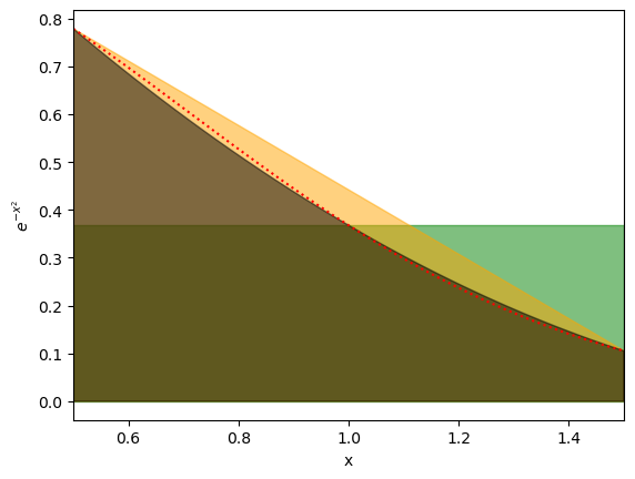
# Let's add the rectangles first. THIS IS CODE FROM BEFORE
num_shapes = 1

edges_x_range = np.linspace(0.5,1.5,num_shapes+1)
x_step = edges_x_range[1] - edges_x_range[0]
intermed_xrange = edges_x_range[:-1] + x_step / 2.
x_range = (edges_x_range[0:-1] + edges_x_range[1:]) / 2. # Can you figure out what this line is doing??
y_vals = np.exp(-x_range**2)
y_vals_trapezium = np.exp(-edges_x_range**2)
y_vals_intermediate = np.exp(-intermed_xrange**2)

# Plot the actual line
full_x_range = np.linspace(0.5,1.5,100000)
full_y_vals = np.exp(-full_x_range**2)
plt.plot(full_x_range, full_y_vals, 'r:') # Plot the line

# plot the rectangles
for x,y in zip(x_range, y_vals): # zip lets me iterate over two lists together
    plt.fill([x-x_step/2, x-x_step/2, x+x_step/2, x+x_step/2],
             [0, y, y, 0], alpha=0.5, color='green', linestyle='-')
plt.plot()

# Now let's add the trapeziums.
for i in range(len(edges_x_range) - 1):
    # Identify the corners of the trapezium, a left edge, right edge, topleft y value, topright y value and bottom y value (0 in all cases)
    left_edge = edges_x_range[i]
    right_edge = edges_x_range[i+1]
    bottom_y_value = 0
    topleft_y_value = y_vals_trapezium[i]
    topright_y_value = y_vals_trapezium[i+1]
    # Draw the trapezium
    plt.fill([left_edge, left_edge, right_edge, right_edge],
             [bottom_y_value, topleft_y_value, topright_y_value, bottom_y_value], alpha=0.5, color='orange', linestyle='-')


# NOW we add the quadrature fits. This is the new code
for i in range(len(edges_x_range) - 1):
    # We have 3 values of x here, the two end points, and the midpoint
    left_edge = edges_x_range[i]
    right_edge = edges_x_range[i+1]
    midpoint = edges_x_range[i] + x_step/2.
    # And the value of the function at end point
    y_val_at_left = y_vals_trapezium[i]
    y_val_at_right = y_vals_trapezium[i+1]
    y_val_at_middle = y_vals_intermediate[i]
    # Then we need to solve y = ax^2 + bx + c. As we have 3 points this is simulataneous equations and we use matrix inversion
    matrix = np.array([[left_edge**2, left_edge, 1],
                       [midpoint**2, midpoint, 1],
                       [right_edge**2, right_edge, 1]])
    inv_matrix = np.linalg.inv(matrix) # Inverts a matrix
    a, b, c = inv_matrix @ np.array([y_val_at_left, y_val_at_middle, y_val_at_right]) # The @ operator is new!!! It does matrix multiplication on numpy arrays
    # Then create a list of points to plot
    curr_x_range = np.linspace(left_edge, right_edge, 1000)
    curr_y_vals = a*curr_x_range**2 + b*curr_x_range + c
    # Add the bottom of the "shape" to integrate
    curr_x_range = [left_edge] + list(curr_x_range) + [right_edge, left_edge]
    curr_y_vals = [0] + list(curr_y_vals) + [0,0]
    plt.fill(curr_x_range, curr_y_vals, alpha=0.5, color='black', linestyle='-')

plt.xlabel('x')
plt.ylabel('$e^{-x^2}$')
plt.xlim(0.5,1.5)

(0.5, 1.5)