Trapezium rule and Simpson’s rule - Solutions

STEP 1

We do need a function to compute the area of a trapezium. Write a function compute_trapeze_area(height_at_left, height_at_right, width). Note that the area of a trapeze is (height_at_left + height_at_right)/2 * width.

import numpy as np
import matplotlib.pyplot as plt

def compute_trapeze_area(height_at_left, height_at_right, width):
    # Complete function here
    return (height_at_left + height_at_right) / 2. * width

# One example to test this
example_area = compute_trapeze_area(3,2,2)
print("Should be 5.0")
print(f"Value computed was {example_area}")

Should be 5.0
Value computed was 5.0

STEP 2

We now have everything we need (we’re deliberately using fewer steps here than when we introduced the rectangle rule). Write a function compute_trapeze_integral(function, lower_val, upper_val, num_rectangles). The function should be the function to compute (ie. compute_ex2) in the example above, lower_val is the lower value of integration, upper_val is the upper value and num_trapeziums is the number of trapeziums to use. Here’s roughly how this should work:

1. Call rectangle_edges to get the edges of your trapeziums (maybe rename the function if you want to avoid the confusion of calling something with rectangle in the name)

2. Call compute_step_size to get the step size.

3. Call function to get the y_values (the heights) of your trapeziums at all the edges.

4. For all trapeziums use compute_trapeze_area to compute the area.

5. Sum over all trapezium areas.

6. Return the integral.

def trapezium_edges(N, lower_val, upper_val): # copied from previous, but name changed
    x_values = np.linspace(lower_val, upper_val, N)
    return x_values

def compute_step_size(trap_edges):
    return trap_edges[1] - trap_edges[0]

def compute_ex2(x_values):
    return np.exp(- x_values**2)

def compute_trapeze_integral(function, lower_val, upper_val, num_trapeziums):
    trap_edges = trapezium_edges(num_trapeziums+1, lower_val, upper_val)
    stepsize = compute_step_size(trap_edges)
    y_values = function(trap_edges)
    areas = compute_trapeze_area(y_values[:-1], y_values[1:], stepsize)
    return np.sum(areas)

# Checking that it works
integral = compute_trapeze_integral(compute_ex2, 0.5, 2, 5)
print("Integral should be 0.4261447643956601")
print(f"Integral was computed to be {integral}")

Integral should be 0.4261447643956601
Integral was computed to be 0.4261447643956601

Exercise

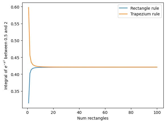
Make a plot of the accuracy of the integral of \(e^{-x^2}dx\) between \(x=0.5\) and \(x=2\) computed using the “rectangle rule” and using the trapezium rule. Plot both on the same plot using two different lines.

The x-axis of the plot should be the number of rectangles used in the integral vary this between 1 rectangle and 100 rectangles. The y-axis should show the value of the integral.

HINT As before, you don’t need to write any integration code here, by this stage you’ve already written it all!

rect_integral_list_ex2 = [0.3144170807266467, 0.40226990312386074, 0.41308241713298993, 0.4165522085393729, 0.4181083032593553, 0.41894082588235804, 0.41943854615366943, 0.41975988647889984, 0.4199794284472106, 0.420136083977214, 0.4202517871569165, 0.4203396728984657, 0.42040799942935114, 0.42046217137315095, 0.4205058467893739, 0.4205415734959833, 0.4205711703587752, 0.42059596405710226, 0.4206169407248601, 0.4206348457397349, 0.4206502509823336, 0.4206636011465935, 0.42067524624143, 0.42068546479747904, 0.4206944806978831, 0.42070247555968837, 0.42070959796131263, 0.4207159704020785, 0.4207216946092978, 0.42072685562662393, 0.42073152499337935, 0.42073576323876505, 0.42073962185462843, 0.4207431448677929, 0.420746370102209, 0.4207493301989571, 0.4207520534457769, 0.42075456445571785, 0.4207568847254853, 0.4207590330972486, 0.420761026142529, 0.42076287848284183, 0.4207646030587309, 0.4207662113564653, 0.42076771359985243, 0.42076911891317265, 0.42077043546009235, 0.42077167056252907, 0.4207728308026966, 0.42077392211100656, 0.4207749498420215, 0.4207759188402755, 0.4207768334974816, 0.42077769780239327, 0.4207785153843706, 0.42077928955155797, 0.4207800233243956, 0.4207807194651442, 0.42078138050391395, 0.42078200876169225, 0.42078260637075277, 0.42078317529276826, 0.4207837173349381, 0.420784234164351, 0.42078472732083083, 0.42078519822841076, 0.42078564820563563, 0.42078607847479804, 0.4207864901702437, 0.4207868843458698, 0.4207872619818617, 0.4207876239908093, 0.4207879712232073, 0.42078830447247667, 0.42078862447948256, 0.4207889319366677, 0.42078922749179765, 0.4207895117513808, 0.42078978528376815, 0.42079004862201885, 0.4207903022664767, 0.4207905466871705, 0.42079078232597256, 0.4207910095986147, 0.4207912288965101, 0.42079144058844903, 0.4207916450221471, 0.42079184252567303, 0.4207920334087667, 0.42079221796405536, 0.42079239646817407, 0.4207925691828022, 0.4207927363556325, 0.4207928982212434, 0.4207930550019355, 0.420793206908486, 0.4207933541408684, 0.42079349688890494, 0.42079363533287456, 0.42079376964408877]
# rect_integral_list copied from previous
trap_integral_list = []
for num_rectangles in range(1, 101):
    #rect_integral_list.append(compute_rectangle_integral(compute_ex2, 0.5, 2, num_rectangles))
    trap_integral_list.append(compute_trapeze_integral(compute_ex2, 0.5, 2, num_rectangles))

plt.plot(range(1,101), rect_integral_list_ex2, label='Rectangle rule')
plt.plot(range(1,101), trap_integral_list, label='Trapezium rule')
plt.xlabel("Num rectangles")
plt.ylabel(r"Integral of $e^{-x^2}$ between 0.5 and 2")
plt.legend()
plt.show()

Exercise

Again, repeat the process for the other two integrals:

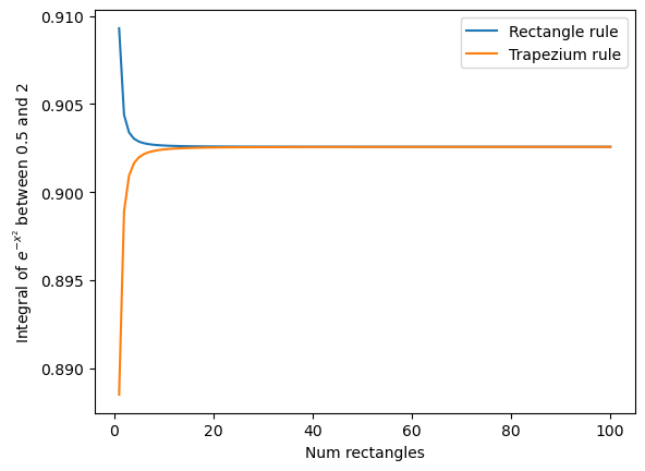
Make a plot of the accuracy of \(\int_1^3\frac{\sin{x}}{x} dx\) computed using the “rectangle rule”, and the “trapezium rule”.

The x-axis of the plot should be the number of rectangles/trapeziums used in the integral vary this between 1 and 100 shapes. The y-axis should show the value of the integral.

HINT All you have to do is copy the previous solution and change the function used, and the range used. I computed the integral to be roughly 0.90257.

def sinc(x_values):
    return np.sin(x_values) / x_values

rect_integral_list_sinc = [0.9092974268256817, 0.904385515377619, 0.9033862496158365, 0.9030307522160774, 0.9028652282287184, 0.902775057322324, 0.9027206003315867, 0.9026852208380283, 0.9026609489754476, 0.9026435795829132, 0.9026307239754605, 0.9026209438298127, 0.9026133311416681, 0.9026072898133084, 0.902602415401979, 0.9025984256708982, 0.902595118818477, 0.9025923474618903, 0.9025900019332169, 0.9025879992647904, 0.9025862757524618, 0.902584781827737, 0.9025834784544708, 0.9025823345532934, 0.9025813251319593, 0.9025804299088317, 0.9025796322863043, 0.902578918576032, 0.9025782774077981, 0.9025776992739187, 0.90257717617477, 0.9025767013406085, 0.902576269011454, 0.9025758742616111, 0.9025755128587482, 0.9025751811499988, 0.902574875969298, 0.9025745945615691, 0.9025743345203145, 0.902574093736008, 0.902573870353182, 0.9025736627345743, 0.9025734694310431, 0.9025732891562112, 0.9025731207650239, 0.9025729632354961, 0.9025728156532018, 0.9025726771979454, 0.902572547132362, 0.9025724247920736, 0.9025723095771874, 0.902572200944926, 0.9025720984032277, 0.9025720015051675, 0.9025719098440743, 0.9025718230492532, 0.9025717407822371, 0.9025716627334843, 0.9025715886194579, 0.9025715181800632, 0.9025714511763202, 0.9025713873883856, 0.9025713266137165, 0.9025712686654759, 0.9025712133710683, 0.9025711605708968, 0.902571110117169, 0.9025710618728725, 0.9025710157108756, 0.9025709715130408, 0.9025709291694998, 0.9025708885779519, 0.9025708496430725, 0.902570812275902, 0.9025707763934079, 0.9025707419179673, 0.9025707087769529, 0.9025706769023812, 0.9025706462305413, 0.9025706167016724, 0.9025705882596895, 0.9025705608518823, 0.9025705344287286, 0.9025705089436082, 0.9025704843526534, 0.9025704606145181, 0.9025704376902068, 0.9025704155429491, 0.902570394138019, 0.9025703734425974, 0.9025703534256834, 0.9025703340579398, 0.9025703153115772, 0.9025702971603098, 0.9025702795792201, 0.9025702625446547, 0.9025702460342105, 0.9025702300266039, 0.9025702145016075, 0.9025701994400331]
# rect_integral_list copied from previous
trap_integral_list = []
for num_shapes in range(1, 101):
    #rect_integral_list.append(compute_rectangle_integral(sinc, 1, 3, num_shapes))
    trap_integral_list.append(compute_trapeze_integral(sinc, 1, 3, num_shapes))

plt.plot(range(1,101), rect_integral_list_sinc, label='Rectangle rule')
plt.plot(range(1,101), trap_integral_list, label='Trapezium rule')
plt.xlabel("Num rectangles")
plt.ylabel(r"Integral of $e^{-x^2}$ between 0.5 and 2")
plt.legend()
plt.show()

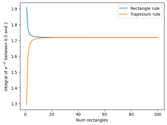
Make a plot of the accuracy of \(\int_1^3 \sqrt{\sin{x}} dx\) computed using the “rectangle rule”, and the “trapezium rule”

The x-axis of the plot should be the number of rectangles/trapeziums used in the integral vary this between 1 and 100 shapes. The y-axis should show the value of the integral.

I computed the integral to be 1.717835 here.

def root_sin(x_values):
    return (np.sin(x_values))**(0.5)

rect_integral_list_rootsin = [1.9071417638190211, 1.7723565217937542, 1.7437729029117706, 1.7329954111513168, 1.727770661488054, 1.724842617602482, 1.7230375411639167, 1.7218466581941605, 1.7210199816151037, 1.7204229203517831, 1.7199777632075626, 1.7196370867075335, 1.719370618598097, 1.7191582997051678, 1.718986412748108, 1.7188453208416572, 1.7187280937317764, 1.71862964473444, 1.7185461723945057, 1.7184747898477504, 1.7184132730979522, 1.7183598865329102, 1.7183132597415105, 1.7182722990956907, 1.71823612332364, 1.718204015915369, 1.7181753895178602, 1.718149758989429, 1.7181267207884428, 1.7181059370506904, 1.718087123175326, 1.7180700380632599, 1.7180544763797039, 1.7180402623752742, 1.7180272449169796, 1.7180152934659012, 1.7180042948009258, 1.7179941503345943, 1.7179847739018166, 1.7179760899287055, 1.717968031908631, 1.717960541127982, 1.7179535655959823, 1.71794705914205, 1.7179409806514272, 1.717935293415304, 1.7179299645764123, 1.7179249646542096, 1.7179202671370297, 1.717915848130513, 1.7179116860536578, 1.7179077613752525, 1.7179040563846877, 1.7179005549921107, 1.7178972425536898, 1.7178941057184627, 1.7178911322937904, 1.7178883111268595, 1.7178856320000748, 1.7178830855385634, 1.717880663128065, 1.7178783568421727, 1.7178761593774239, 1.7178740639955004, 1.717872064471519, 1.7178701550478772, 1.7178683303927191, 1.7178665855627375, 1.7178649159697463, 1.7178633173504256, 1.7178617857391631, 1.7178603174434266, 1.7178589090215548, 1.7178575572624928, 1.717856259167625, 1.7178550119340337, 1.7178538129393859, 1.7178526597282013, 1.7178515499992437, 1.7178504815940254, 1.7178494524863517, 1.7178484607726412, 1.7178475046632373, 1.7178465824742115, 1.7178456926200598, 1.7178448336068037, 1.717844004025728, 1.71784320254767, 1.7178424279176323, 1.7178416789498685, 1.7178409545234132, 1.7178402535778188, 1.7178395751092563, 1.7178389181670255, 1.7178382818501456, 1.7178376653042287, 1.7178370677187385, 1.7178364883242145, 1.7178359263898093, 1.71783538122107]
# copied from previous
trap_integral_list = []
for num_shapes in range(1, 101):
    #rect_integral_list.append(compute_rectangle_integral(root_sin, 1, 3, num_shapes))
    trap_integral_list.append(compute_trapeze_integral(root_sin, 1, 3, num_shapes))

plt.plot(range(1,101), rect_integral_list_rootsin, label='Rectangle rule')
plt.plot(range(1,101), trap_integral_list, label='Trapezium rule')
plt.xlabel("Num rectangles")
plt.ylabel(r"Integral of $e^{-x^2}$ between 0.5 and 2")
plt.legend()
plt.show()

Simpson’s rule

We have now demonstrated both the rectangular and trapezium integration methods. While the trapezium method looks like a visibly better fit, there are cases (including the cases above) where the rectangle method is actually more accurate. However, this can be improved by using a “2nd-order” solution to the problem.

Simpson’s rule is that. In this case rather than assuming that the curve is a series of straight lines, we assume that the curve is a series of quadratic lines. A nice introduction to this can be seen here:

https://web.stanford.edu/group/sisl/k12/optimization/MO-unit4-pdfs/4.2simpsonintegrals.pdf

(see up to slide 7). Let’s try and visualize how this will look for our \(e^{-x^2}dx\). Here I will compare to using only one rectangle/trapezium to emphasize the difference.

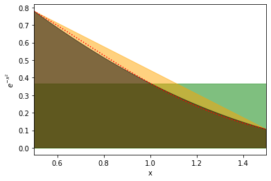
Here the red is the actual curve, the green is the rectangle, the orange the trapezium, and the black is the new quadrature fit. We can see that each is progressively fitting better.

Now we just need to evaluate this integral. Now we could analytically integrate the quadratic curve at every point, but it turns out that the integral of a quadratic curve over the interval \(a\) to \(b\) (where the midpoint is \(m\)) is given by:

\[\int_a^b f(x) dx \approx \frac{(b-a)}{6}\left(f(a)+4f(m) + f(b) \right) \]

We can code this up.

Step 1

Write a function compute_quadrature_area(height_at_left, height_at_middle, height_at_right, width) to compute the area of the shapes used in Simpson’s rule. As described above this function should return width/6. * (height_at_left + 4*height_at_middle + height_at_right)

def compute_quadrature_area(height_at_left, height_at_middle, height_at_right, width):
    # Complete function below
    return width / 6. * (height_at_left + 4 * height_at_middle + height_at_right)


# One example to test this
example_area = compute_quadrature_area(3,2,3,2)
print("Should be 4.666666666666666")
print(f"Value computed was {example_area}")

Should be 4.666666666666666
Value computed was 4.666666666666666

Step 2

Now we can write a function compute_simpsons_integral(function, lower_val, upper_val, num_rectangles). The function should be the function to compute (ie. compute_ex2) in the example above, lower_val is the lower value of integration, upper_val is the upper value and num_trapeziums is the number of trapeziums to use. Here’s roughly how this could work:

1. Call rectangle_edges to get the edges of your shapes (maybe rename the function if you want to avoid the confusion of calling something with rectangle in the name)

2. Call compute_step_size to get the step size.

3. Call f_midpoints to get the midpoints of your shapes

4. Call function to get the y_values (the heights) of your shapes at all the edges.

5. Call function again to get the y_values of the shapes at all the midpoints.

6. For all shapes use compute_quadrature_area to compute the area.

7. Sum over all areas.

8. Return the integral.

def f_midpoints(lower_edge, upper_edge):
    return (upper_edge + lower_edge)/2

def compute_simpsons_integral(function, lower_val, upper_val, num_shapes):
    shape_edges = trapezium_edges(num_shapes+1, lower_val, upper_val)
    stepsize = compute_step_size(shape_edges)
    trap_midpoints = f_midpoints(shape_edges[:-1], shape_edges[1:])
    y_values_at_edges = function(shape_edges)
    y_values_at_midpoints = function(trap_midpoints)
    areas = compute_quadrature_area(y_values_at_edges[:-1], y_values_at_midpoints, y_values_at_edges[1:], stepsize)
    return np.sum(areas)


# Checking that it works
integral = compute_simpsons_integral(compute_ex2, 0.5, 2, 5)
print("Integral should be 0.4207871236381236")
print(f"Integral was computed to be {integral}")

Integral should be 0.4207871236381236
Integral was computed to be 0.4207871236381236

Some optimization

If we examine this closely (with 2 shapes), we can see that the right edge of the first shape is the left edge of the second shape, therefore we don’t need to compute that twice. We can just compute the value of the function at all the points we need (which will be twice as many points as with the trapezium rule, as we need to compute midpoints). Then we just multiply each point by a weighting. This weighting will be 4 for all the midpoints, 1 for the first and last point, and 2 otherwise. So for example if we were doing this with 3 shapes we would do something like:

\[\begin{split} \begin{array}{|c|c|c|}\hline x & f(x) & \mbox{weight} \\ \hline 0.5 & 0.778801 & 1\\ 0.666667 & 0.641180 & 4\\ 0.833333 & 0.499352 & 2\\ 1 & 0.367880 & 4\\ 1.166667 & 0.256376 & 2\\ 1.333333 & 0.169013 & 4\\ 1.5 & 0.105399 & 1\\ \hline \end{array} \end{split}\]

Then we just multiply all the f(x) values by the weights and sum everything up.

Integral = (0.778801 + 0.641180*4 + 0.499352*2 + 0.367880*4 + 0.256376*2 + 0.169013*4 + 0.105399) * width / 6.

def simpson_rule(function, lower_val, upper_val, num_shapes):
    h = (upper_val - lower_val)/num_shapes
    x_vals = np.linspace(lower_val, upper_val, num_shapes*2+1)
    f_vals = function(x_vals)
    weights = np.ones(len(f_vals)) # Start with all weights equal to 1, then use slicing magic
    weights[1::2] = 4 # Set every other value, starting with the second, to 4
    weights[2:-1:2] = 2 # Set every other value, starting with the third, and not including the last, to 2
    #print(weights) # Definitely use a debug statement here to check we got what we expected!!
    return h/6*np.sum(f_vals*weights)

current_area = simpson_rule(compute_ex2, 0.5, 2, 5)

print(f"I have computed the integral to be {current_area} with numerical integration using Simpson's rule")

I have computed the integral to be 0.42078712363812343 with numerical integration using Simpson's rule

Exercise

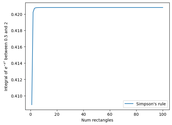
Make a plot of the accuracy of the integral of \(e^{-x^2}dx\) between \(x=0.5\) and \(x=2\) computed using Simpson’s rule.

The x-axis of the plot should be the number of shapes used in the integral. Vary this between 1 shape and 100 shapes. The y-axis should show the value of the integral.

HINT As before, you don’t need to write any integration code here, it’s all provided above.

#rect_integral_list = []
#trap_integral_list = []
simp_integral_list = []
for num_shapes in range(1, 101):
    #rect_integral_list.append(compute_rectangle_integral(compute_ex2, 0.5, 2, num_shapes))
    #trap_integral_list.append(compute_trapeze_integral(compute_ex2, 0.5, 2, num_shapes))
    simp_integral_list.append(compute_simpsons_integral(compute_ex2, 0.5, 2, num_shapes))

#plt.plot(range(1,101), rect_integral_list_ex2, label='Rectangle rule')
#plt.plot(range(1,101), trap_integral_list, label='Trapezium rule')
plt.plot(range(1,101), simp_integral_list, label="Simpson's rule")
plt.xlabel("Num rectangles")
plt.ylabel(r"Integral of $e^{-x^2}$ between 0.5 and 2")
plt.legend()
plt.show()

Exercise

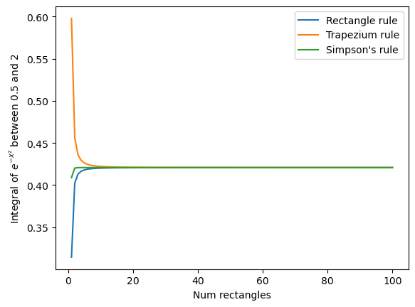
TL:DR: Now repeat the process but plot the accuracy using Simpson’s rule, Trapezium rule and rectangle rule on the same plot!

Longer: Make a plot of the accuracy of the integral of \(e^{-x^2}dx\) between \(x=0.5\) and \(x=2\) computed using Simpson’s rule, Trapezium rule and the Rectangle rule. Show the 3 lines on the same plot.

The x-axis of the plot should be the number of shapes used in the integral. Vary this between 1 shape and 100 shapes. The y-axis should show the value of the integral.

HINT As before, you don’t need to write any integration code here, it’s all provided above.

#rect_integral_list = []
trap_integral_list = []
simp_integral_list = []
for num_shapes in range(1, 101):
    #rect_integral_list.append(compute_rectangle_integral(compute_ex2, 0.5, 2, num_shapes))
    trap_integral_list.append(compute_trapeze_integral(compute_ex2, 0.5, 2, num_shapes))
    simp_integral_list.append(compute_simpsons_integral(compute_ex2, 0.5, 2, num_shapes))

plt.plot(range(1,101), rect_integral_list_ex2, label='Rectangle rule')
plt.plot(range(1,101), trap_integral_list, label='Trapezium rule')
plt.plot(range(1,101), simp_integral_list, label="Simpson's rule")
plt.xlabel("Num rectangles")
plt.ylabel(r"Integral of $e^{-x^2}$ between 0.5 and 2")
plt.legend()

<matplotlib.legend.Legend at 0x11894ca30>

Exercise

Again, repeat the process for the other two integrals:

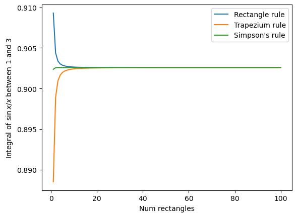
Make a plot of the accuracy of \(\int_1^3\frac{\sin{x}}{x} dx\) computed using the “rectangle rule”, the “trapezium rule” and “Simpson’s rule”

The x-axis of the plot should be the number of shapes used in the integral vary this between 1 and 100 shapes. The y-axis should show the value of the integral.

HINT All you have to do is copy the previous solution and change the function used, and the range used. I computed the integral to be roughly 0.90257.

#rect_integral_list = []
trap_integral_list = []
simp_integral_list = []
for num_shapes in range(1, 101):
    #rect_integral_list.append(compute_rectangle_integral(sinc, 1, 3, num_shapes))
    trap_integral_list.append(compute_trapeze_integral(sinc, 1, 3, num_shapes))
    simp_integral_list.append(compute_simpsons_integral(sinc, 1, 3, num_shapes))

plt.plot(range(1,101), rect_integral_list_sinc, label='Rectangle rule')
plt.plot(range(1,101), trap_integral_list, label='Trapezium rule')
plt.plot(range(1,101), simp_integral_list, label="Simpson's rule")
plt.xlabel("Num rectangles")
plt.ylabel(r"Integral of $\sin{x} / x$ between 1 and 3")
plt.legend()

<matplotlib.legend.Legend at 0x1189688e0>

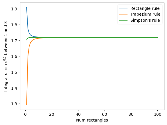
Make a plot of the accuracy of \(\int_1^3 \sqrt{\sin{x}} dx\) computed using the “rectangle rule”, the “trapezium rule” and “Simpson’s rule”

The x-axis of the plot should be the number of shapes used in the integral vary this between 1 and 100 shapes. The y-axis should show the value of the integral.

I computed the integral to be 1.717835 here.

#rect_integral_list = []
trap_integral_list = []
simp_integral_list = []
for num_shapes in range(1, 101):
    #rect_integral_list.append(compute_rectangle_integral(root_sin, 1, 3, num_shapes))
    trap_integral_list.append(compute_trapeze_integral(root_sin, 1, 3, num_shapes))
    simp_integral_list.append(compute_simpsons_integral(root_sin, 1, 3, num_shapes))

plt.plot(range(1,101), rect_integral_list_rootsin, label='Rectangle rule')
plt.plot(range(1,101), trap_integral_list, label='Trapezium rule')
plt.plot(range(1,101), simp_integral_list, label="Simpson's rule")
plt.xlabel("Num rectangles")
plt.ylabel(r"Integral of $\sin{x}^{0.5}$ between 1 and 3")
plt.legend()
plt.show()

Exercise

Compute the integral:

\[\int_{0.2}^{0.5} \tan(x) dx\]

using numerical integration

compute_simpsons_integral(np.tan, 0.2, 0.5, 100000)

0.11044946739142483

Exercise

Compute the integral

\[\int_0^{20} e ^ {\sin(x)} dx \]

def esinx(x):
    return np.exp(np.sin(x))

compute_simpsons_integral(esinx, 0, 20, 100000)

25.85902105079306

Exercise

Compute the integral

\[\int_1^{100} \frac{\ln (x + 1)}{x} dx \]

def lnweirdness(x):
    return np.log(x + 1) / x

compute_simpsons_integral(lnweirdness, 1, 100, 100000)

11.41628814389136

Exercise

Compute the integral:

\[\int_{1}^{2} \tan(x) dx\]

using numerical integration.

WARNING There’s a catch in this one! Maybe try plotting \(\tan(x)\) in this internal first?? If you can see the catch, is it still possible to integrate this?

# tan(x) goes to infinity at x = pi/2. The integral also tends to infinity if the upper limit is pi/2.
# However, one can use a symmetry argument. Over a complete cycle there is equal area below 0 as above 0,
# and so the integral of tan(x) from pi/2 to 2 is equal to the negative of the integral of tan(x) from
# pi/2 - (2 - pi/2) to pi/2. So we *can* compute this, by removing this section and just integrating from
# 1 to pi - 2.
compute_simpsons_integral(np.tan, 1, np.pi-2, 100000)

0.2610906381273086