The Trapezium rule
Contents
The Trapezium rule#
The rectangle rule is a “0th order” solution for numerical integration. Let’s now consider a “1st order” solution. The difference is that with rectangles we are assuming that the value of the function is constant over the rectangle and jumps to a new value when we get to next one. What if instead the function varied (in a straight line) between each point. To do that we use trapeziums instead of rectangles, and we need to evaluate the value of the function at the edge of each trapezium not in the middle.
Let’s visualize what this would look like with 3 trapeziums, and compare to the rectangles used previously (we use a small number of shapes to make it easier to see the trapeziums)
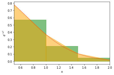
Here the red line is the actual curve, the green is the rectangles used in the rectangular method, and the yellow is the area used in the trapezium rule. It looks like the yellow and red agree almost perfectly.
As before to compute the integral we need to compute the area of each of the trapeziums and sum them up to get an approximation of the integral. If you are happy to try this out on your own, please proceed below. Otherwise we will guide you through the differences between this and the rectangle approach.
import numpy as np
import matplotlib.pyplot as plt
One thing to highlight here is that there are a lot of similarities between the trapezium and rectangle approaches. The shapes have the same positions on the x-axis so we can re-use a lot of code from before. We do not compute any “midpoints” here, but stepsize and rectangle_edges can be used directly. (Copy them into this workbook)
STEP 1#
We do need a function to compute the area of a trapezium. Write a function compute_trapeze_area(height_at_left, height_at_right, width). Note that the area of a trapeze is (height_at_left + height_at_right)/2 * width.
def compute_trapeze_area(height_at_left, height_at_right, width):
    # Complete function here


# One example to test this
example_area = compute_trapeze_area(3,2,2)
print("Should be 5.0")
print(f"Value computed was {example_area}")
  Input In [2]
    example_area = compute_trapeze_area(3,2,2)
    ^
IndentationError: expected an indented block
STEP 2#
We now have everything we need (we’re deliberately using fewer steps here than when we introduced the rectangle rule). Write a function compute_trapeze_integral(function, lower_val, upper_val, num_rectangles). The function should be the function to compute (ie. compute_ex2) in the example above, lower_val is the lower value of integration, upper_val is the upper value and num_trapeziums is the number of trapeziums to use. Here’s roughly how this should work:
Call
rectangle_edgesto get the edges of your trapeziums (maybe rename the function if you want to avoid the confusion of calling something with rectangle in the name)Call
compute_step_sizeto get the step size.Call
functionto get the y_values (the heights) of your trapeziums at all the edges.For all trapeziums use
compute_trapeze_areato compute the area.Sum over all trapezium areas.
Return the integral.
def compute_trapeze_integral(function, lower_val, upper_val, num_trapeziums):
    # Complete function below


# Checking that it works
integral = compute_trapeze_integral(compute_ex2, 0.5, 2, 5)
print("Integral should be 0.4261447643956601")
print(f"Integral was computed to be {integral}")
  Input In [3]
    integral = compute_trapeze_integral(compute_ex2, 0.5, 2, 5)
    ^
IndentationError: expected an indented block
Exercise#
Make a plot of the accuracy of the integral of \(e^{-x^2}dx\) between \(x=0.5\) and \(x=2\) computed using the “rectangle rule” and using the trapezium rule. Plot both on the same plot using two different lines.
The x-axis of the plot should be the number of rectangles used in the integral vary this between 1 rectangle and 100 rectangles. The y-axis should show the value of the integral.
HINT As before, you don’t need to write any integration code here, by this stage you’ve already written it all!
# ADD CODE HERE
Exercise#
Again, repeat the process for the other two integrals:
Make a plot of the accuracy of \(\int_1^3\frac{\sin{x}}{x} dx\) computed using the “rectangle rule”, and the “trapezium rule”.
The x-axis of the plot should be the number of rectangles/trapeziums used in the integral vary this between 1 and 100 shapes. The y-axis should show the value of the integral.
HINT All you have to do is copy the previous solution and change the function used, and the range used. I computed the integral to be roughly 0.90257.
# ADD CODE HERE
Make a plot of the accuracy of \(\int_1^3 \sqrt{\sin{x}} dx\) computed using the “rectangle rule”, and the “trapezium rule”
The x-axis of the plot should be the number of rectangles/trapeziums used in the integral vary this between 1 and 100 shapes. The y-axis should show the value of the integral.
I computed the integral to be 1.717835 here.
# ADD CODE HERE