Introduction

By this point you have seen in many places in your maths/physics degree how important integration and differentiation are in solving many problems.

However, there is an important difference between integration and differentiation. Namely, differentiation is much easier than integration in the general case. The reason for this is that you have learned by now a set of rules (chain rule, product rule etc.) which can always be applied step by step to differentiate the vast majority of functions analytically. Sometimes this can take a long time, and it’s easy to make a mistake, but it can still be done (I note that there are mathematical computer “languages” like mathematica/maple that can greatly increase the speed of such analytical approaches, and reduce the chance of making errors).

Integration in contrast is much harder. It generally relies on trying to find a function that differentiates to what you have and saying “that is the integral”. For some cases this is not so bad, but for other cases this can be very difficult.

For this reason it is often easiest to solve an integration problem not by writing hundreds of lines of algebra, but by using a computer and doing it “numerically”. I note that differentials can also be evaluated numerically, but here we focus on integration as this is where the analytic solutions are harder.

For some simple examples of where integration can be hard, consider the following examples:

\[ \int_a^b \sqrt{\sin{x}} dx, \int_a^b \frac{\sin{x}}{x} dx, \ \int_a^b e^{-x^2}dx\]

and try to integrate these on pen and paper without looking up solutions …. Don’t spend too long on this (or indeed, any time on this); there is no compact solution to this beyond writing these out in Taylor expansions and integrating every term.

Numerical solution

Although we can’t write down an algebraic solution to these integrals we can still compute an integral between given limits numerically.

As an example consider the following:

• Compute the integral of \(e^{-x^2}dx\) between \(x=1\) and \(x=3\)

To understand this, first lets try to graphically show what we need to do. We will begin by visualizing \(e^{-x^2}dx\) between \(x=0.5\) and \(x=1.5\)

NOTE: I will be using python to make the graphical illustrations. The code used for these is in the appendix. We will be building up to making your own versions of this stuff later though.

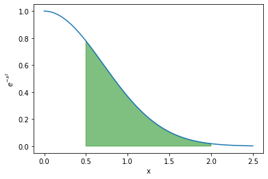
Now, all we need to do is work out the area of the green region in the above plot to compute this integral. We will demonstrate a few ways of doing this, starting from a basic approximation (less accurate, but easier to explain and code) to something more complicated (more accurate, but harder to explain and code). To illustrate this more clearly we will deliberatly use much fewer points on the x-axis than we should.

Rectangle rule

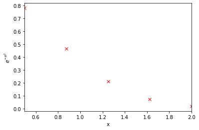
Consider again this function denoted by 5 equally spaced points, now only shown between 0.5 and 2:

At each of these points we draw a rectangle. The rectangles should be centered on the points and must not overlap:

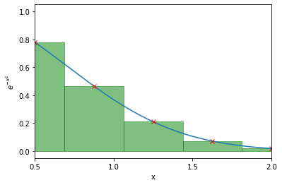
If we then computed the area of each of these rectangles (width * height) and summed them all up, we would have an estimate of the integral! However, in this example the first and last rectangle are only half on the plot, so let’s center this so that all the rectangles have the same width:

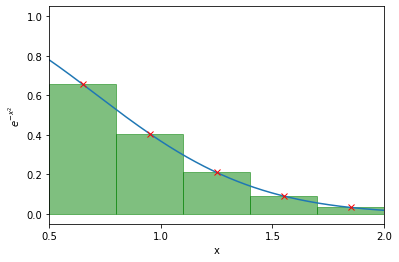
Then if we were to compute the area of these 5 rectangles, and sum it up, we would get 0.4181083032593553. In doing so we have approximately computed \(\int_{0.5}^{2} e^{-x^2} dx\) to be 0.418 (no point quoting this to 21 decimal places with only 5 rectangles).

However, this does approximate the function as a set of 5 horizontal lines, when in reality this is a smooth line. So to get a better approximation we really want to use more, narrower rectangles. Let’s try now with 100 rectangles.

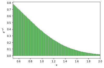
In this case the integral is computed to be 0.4208. The balance here is how many rectangles do we need to compute an accurate integral balanced against how long will it take to compute this.